Interest Rates

Determination, structure, and valuation in capital markets

Dr. Isai Guízar · CUCEA, Department of Economics

August 2026

Interest Rates

Determination, structure, and valuation

Capital Markets · CUCEA
Dr. Isai Guízar · Department of Economics

Based on Mishkin & Eakins, Financial Markets and Institutions, chaps. 3–5

Welcome. Frame the session: why the price of money (the interest rate) is the single most important price in a market economy.

Before we start

Why can the U.S. government borrow at almost zero cost, while a company like Tesla pays several percentage points more for the same maturity?

By the end of the session you’ll be able to answer this with three pieces: present value, supply and demand for bonds, and the risk-and-maturity structure of interest rates.

Roadmap for today

① Valuation

From cash flow to price: credit instruments and present value.

② Determination

Supply and demand for bonds → the level of interest rates.

③ Structure

Why there’s no single rate: risk, liquidity, and maturity.

① Valuation

From cash flows to price

• Every debt instrument promises a different stream of payments (cash flows) over time.
• We can’t compare $1 today with $1 five years from now without adjusting for time → present value.
• Equating the present value of the flows with the market price gives us the implicit interest rate: the yield to maturity (YTM).

Key idea
YTM is the rate that makes what you pay today exactly equal to what the promise of future payments is worth today.

Four credit instruments

1 · Simple loan

A single payment at maturity (principal + interest).

2 · Fixed-payment loan

The same annuity payment every period (mortgage, auto loan).

3 · Coupon bond

Periodic fixed payments (coupon) + face value at maturity.

4 · Discount bond

Bought below face value; a single payment = face value.

All four are the same math problem: discounting future cash flows at a rate \(i\).

Simple loan

Example
Pete borrows $100 from his sister, and a year later pays her back $110. What is the YTM on this loan?

principal, final_payment = 100, 110
ytm_simple = final_payment/principal - 1
print(f"Simple loan YTM = {ytm_simple:.1%}")

Simple loan YTM = 10.0%

For a simple loan, the simple interest rate = the YTM. It’s the easiest case — and the starting point for everything else.

Fixed-payment loan

\[ LV = \frac{FP}{(1+i)} + \frac{FP}{(1+i)^2} + \dots + \frac{FP}{(1+i)^n} \]

Case 1 A $100,000 mortgage at 7% annual interest, 20-year term. What’s the annual payment?

LV, i, n = 100_000, 0.07, 20
annuity_factor = (1 - (1+i)**-n) / i
payment = LV / annuity_factor
print(f"Annual payment = ${payment:,.2f}")

Annual payment = $9,439.29

From rate to APR (a real-world twist)

Case 2 A bank lends $4,000, to be repaid in 12 monthly installments of $370. What is the annual rate (APR)?

LV, payment, n = 4_000, 370, 12
f = lambda i: sum(payment/(1+i)**t for t in range(1, n+1)) - LV
i_monthly = bisect_rate(f, 1e-6, 1.0)
print(f"Monthly rate        = {i_monthly:.4%}")
print(f"APR (i × 12)         = {i_monthly*12:.2%}")
print(f"Effective annual rate = {(1+i_monthly)**12 - 1:.2%}")

Monthly rate        = 1.6432%
APR (i × 12)         = 19.72%
Effective annual rate = 21.60%

APR (annual percentage rate) is the regulatory convention; the effective annual rate is what you actually pay once monthly compounding is accounted for.

Which loan is better? (hidden fees)

Case 3 Juan needs $800,000 over 5 years, fixed monthly payments, 7% nominal rate.
Bank A: $50,000 origination fee.
Bank B: no fee, but an extra $1,000 per month.

loan, nominal_rate, n = 800_000, 0.07, 60
i_m = nominal_rate/12
payment = loan * i_m / (1 - (1+i_m)**-n)

# Bank A: the fee reduces what Juan actually receives
net_proceeds = loan - 50_000
f_bankA = lambda i: sum(payment/(1+i)**t for t in range(1, n+1)) - net_proceeds
apr_bankA = bisect_rate(f_bankA, 1e-6, 1.0) * 12

# Bank B: Juan receives the full amount, but pays an extra monthly fee
payment_B = payment + 1_000
f_bankB = lambda i: sum(payment_B/(1+i)**t for t in range(1, n+1)) - loan
apr_bankB = bisect_rate(f_bankB, 1e-6, 1.0) * 12

print(f"Base monthly payment   = ${payment:,.2f}")
print(f"Effective APR, Bank A  = {apr_bankA:.2%}")
print(f"Effective APR, Bank B  = {apr_bankB:.2%}")
print(f"Total cost, Bank A     = ${payment*n + 50_000:,.0f}")
print(f"Total cost, Bank B     = ${payment_B*n:,.0f}")

Base monthly payment   = $15,840.96
Effective APR, Bank A  = 9.74%
Effective APR, Bank B  = 9.60%
Total cost, Bank A     = $1,000,458
Total cost, Bank B     = $1,010,458

The “advertised” rate (7% in both cases) hides different real costs. Always compare the effective APR, never the nominal rate.

Coupon bond: the general formula

\[ P=\frac{C}{(1+i)}+\frac{C}{(1+i)^2}+\dots+\frac{C}{(1+i)^n}+\frac{F}{(1+i)^n} \]

Example A bond with a 10% coupon, $1,000 face value, 12.25% YTM, and 8 years to maturity.

C, F, y, n = 100, 1000, 0.1225, 8
P = sum(C/(1+y)**t for t in range(1, n+1)) + F/(1+y)**n
print(f"Bond price = ${P:,.2f}   (sells at a discount because YTM > coupon)")

Bond price = $889.20   (sells at a discount because YTM > coupon)

Price and yield: the inverse relationship

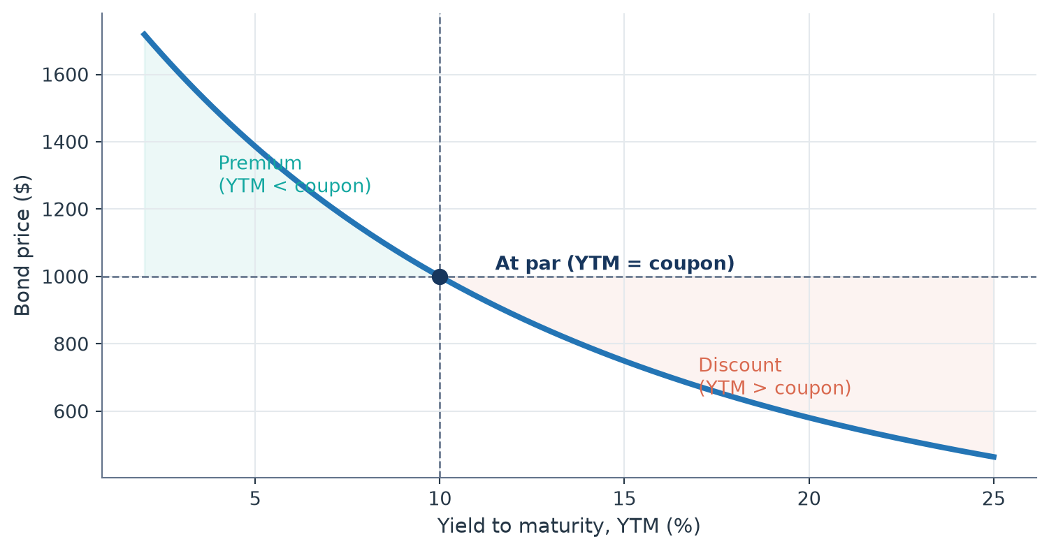
Figure 1: Price of a 10% coupon bond, 10-year maturity (FV = $1,000), by YTM

Memorize the shape, not the table: price and yield always move in opposite directions.

Distinction: interest rate ≠ return

\[ R=\frac{C+P_{t+1}-P_t}{P_t}=i_c+g \]

Example You buy a bond for $1,000 (8% coupon) and sell it a year later for $800. What was your return?

C, Pt, Pt1 = 80, 1000, 800
R = (C + Pt1 - Pt)/Pt
print(f"Realized return = {R:.1%}   ← negative, even though the coupon was 8%!")

Realized return = -12.0%   ← negative, even though the coupon was 8%!

When rates rise: who loses the most?

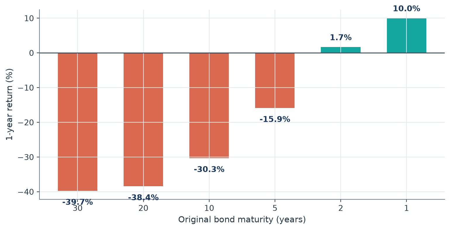
Scenario 10%-coupon bonds (FV $1,000) bought when i = 10%. A year later the rate rises to 20%. One-year return by original maturity.

Figure 2: The longer the maturity, the larger the capital loss when rates rise

Only the bond whose maturity equals your holding period guarantees the initial YTM. Everything else carries interest-rate risk.

Nominal vs. real interest rates

\[ i = r + \pi^{e} \]

• \(i\) = nominal rate (the one that’s quoted)
• \(r\) = real rate (purchasing power)
• \(\pi^{e}\) = expected inflation

With low or negative real rates, it pays to borrow, not to lend — the key to understanding the Japan case we’ll see shortly.

② Determination

The bond market, in one idea

• A bond is simply tradable debt: the issuer borrows, the buyer lends.
• The bond’s price is determined like any market price: supply and demand.
• Since price and rate move in opposite directions, understanding the bond market is understanding what moves interest rates.

Demand for bonds

Zero-coupon bond $1,000 face value, one year to maturity. \(P=\dfrac{FV}{1+i}\)

FV = 1000
for P in [950, 900, 850, 800, 750]:
    print(f"Price ${P}  →  i = {FV/P - 1:.1%}")

Price $950  →  i = 5.3%
Price $900  →  i = 11.1%
Price $850  →  i = 17.6%
Price $800  →  i = 25.0%
Price $750  →  i = 33.3%

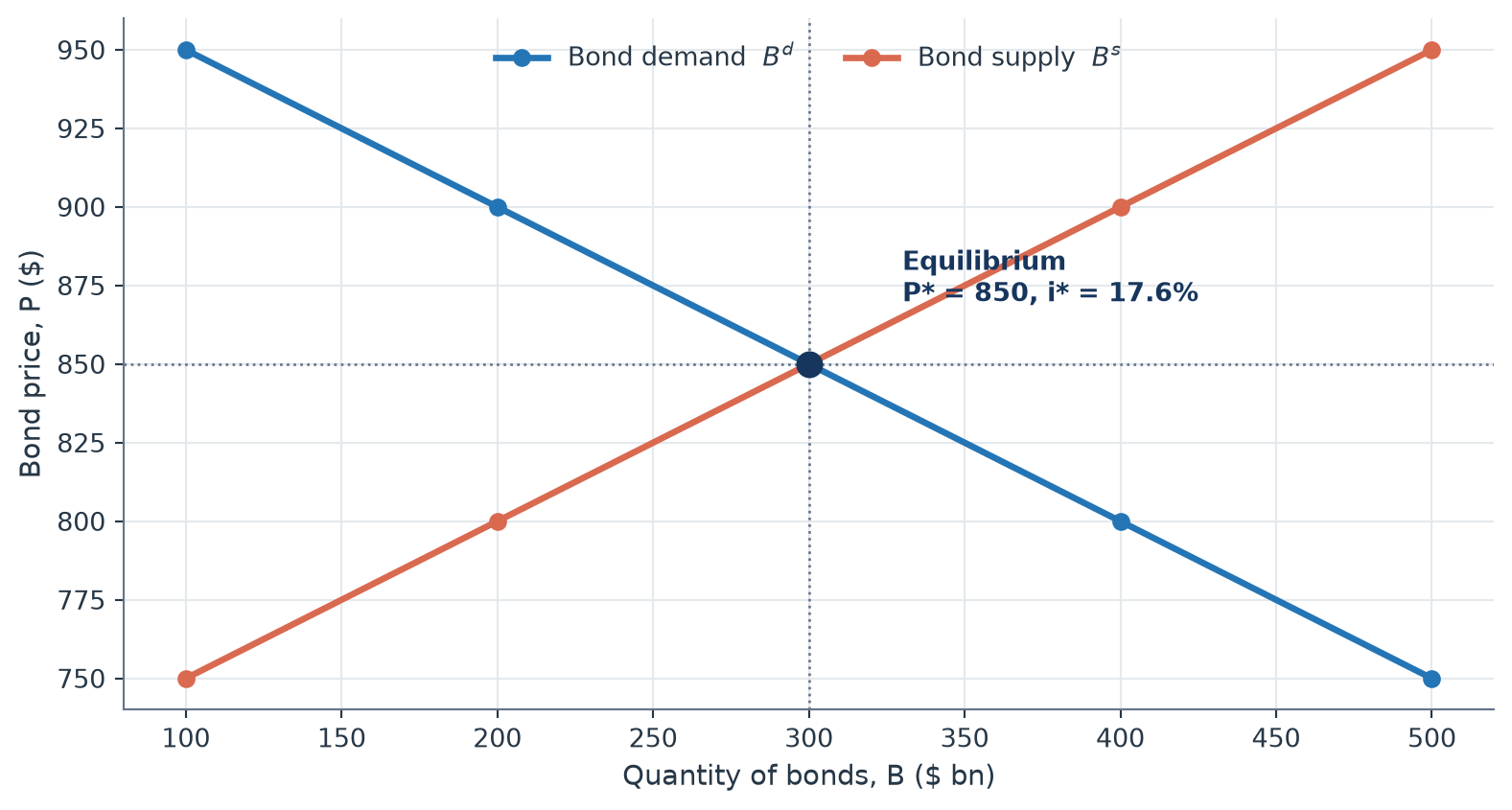
At a lower price, the implicit rate is higher → more attractive to buyers → higher quantity demanded.

Equilibrium in the bond market

Figure 3: Bond supply and demand: equilibrium sets the price (and the rate)

Excess supply → price falls until P*. Excess demand → price rises until P*. The market always “finds” P*.

What shifts the demand for bonds?

• 💰 Wealth ↑ → more savings available → \(B^d\) shifts right
• 📈 Expected return relative to other assets ↑ → \(B^d\) shifts right
• ⚠️ Risk of the bond ↓ (or risk of alternatives ↑) → \(B^d\) shifts right
• 💧 Liquidity of the bond ↑ → \(B^d\) shifts right

Remember: a shift of the curve ≠ a movement along it. The bond’s own price moves the quantity demanded; everything else shifts the whole curve.

What shifts the supply of bonds?

• 🏗️ Investment opportunities (economic expansion) ↑ → \(B^s\) shifts right
• 🔺 Expected inflation ↑ → the real cost of borrowing falls → \(B^s\) shifts right
• 🏛️ Government deficit ↑ → more public debt issuance → \(B^s\) shifts right

Case 1 · Business-cycle expansion

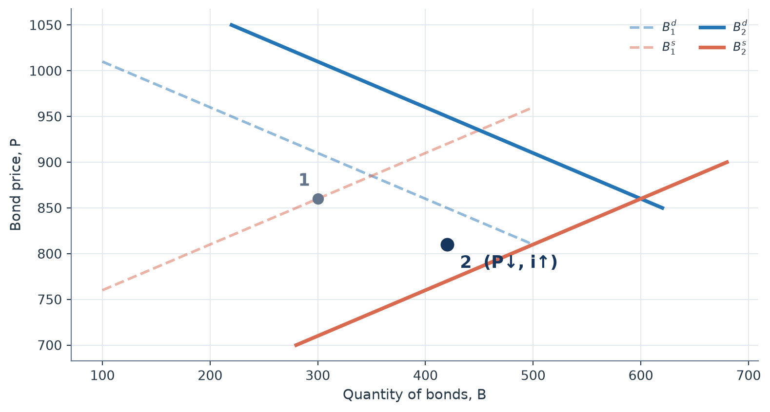
Question In an expansion, national income rises. What happens to the interest rate?

• Wealth ↑ → \(B^d\) shifts to the right
• Investment opportunities ↑ → \(B^s\) shifts to the right, and by more than demand

Figure 4: If supply shifts more than demand: price falls, and the rate rises

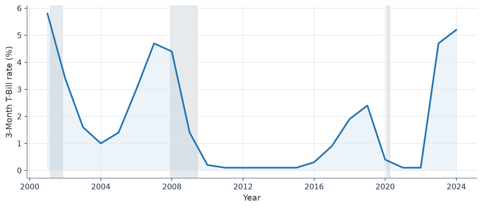
Empirical result: interest rates are procyclical — they rise in expansions and fall in recessions.

Interest rates and the business cycle (live data)

# Pull the real, current series straight from FRED (no API key needed
# for the CSV endpoint). Falls back to a small bundled sample if the
# machine has no internet access at render time.
FRED_URL = "https://fred.stlouisfed.org/graph/fredgraph.csv?id=TB3MS"

try:
    tbill = pd.read_csv(FRED_URL)
    tbill.columns = ["date", "rate"]
    tbill["date"] = pd.to_datetime(tbill["date"])
    tbill["rate"] = pd.to_numeric(tbill["rate"], errors="coerce")
    tbill = tbill.dropna().query("date >= '2000-01-01'")
    x, y = tbill["date"], tbill["rate"]
    source_note = "Source: FRED, series TB3MS (fetched live)."
except Exception as e:
    print(f"Could not reach FRED ({e}); using a small bundled sample instead.")
    x = pd.date_range("2000-01-01", periods=24, freq="YE")
    y = [5.8,3.4,1.6,1.0,1.4,3.0,4.7,4.4,1.4,0.2,0.1,0.1,
         0.1,0.1,0.1,0.3,0.9,1.9,2.4,0.4,0.1,0.1,4.7,5.2]
    source_note = "Source: bundled offline sample (FRED unreachable at render time)."

# NBER recession dates (official, hand-entered — no live lookup needed).
recessions = [
    ("2001-03-01", "2001-11-01"),
    ("2007-12-01", "2009-06-01"),
    ("2020-02-01", "2020-04-01"),
]

fig, ax = plt.subplots(figsize=(9,4))
ax.plot(x, y, color=BLUE, lw=2.2)
ax.fill_between(x, y, color=BLUE, alpha=.08)
for start, end in recessions:
    ax.axvspan(pd.Timestamp(start), pd.Timestamp(end), color=GRAYM, alpha=.15)
brand_axes(ax, xlabel="Year", ylabel="3-Month T-Bill rate (%)")
plt.tight_layout()
plt.show()
print(source_note)

Could not reach FRED (<urlopen error [SSL: CERTIFICATE_VERIFY_FAILED] certificate verify failed: unable to get local issuer certificate (_ssl.c:1082)>); using a small bundled sample instead.

Figure 5: 3-Month U.S. Treasury Bill rate — shaded bands mark NBER recessions

Source: bundled offline sample (FRED unreachable at render time).

This cell fetches the actual, up-to-date series every time you render — no numbers are hardcoded. Re-run it anytime to refresh the chart with the latest data.

Case 2 · Deflation in Japan

Context From the late 1990s through the 2010s, Japan experienced low/negative inflation and near-zero interest rates. How does the model explain it?

• Expected inflation ↓ → the real return on bonds ↑ → \(B^d\) shifts right
• Expected inflation ↓ → the real cost of borrowing ↑ → \(B^s\) shifts left
• Both effects push the price up → the rate falls. ✅ Consistent with the evidence.

③ Structure

There is no single “interest rate”

• Bonds with similar cash flows but different prices → differences explained by risk (risk structure).
• Bonds with the same risk but different maturities → differences explained by the yield curve (term structure).

Default risk

• The risk premium = the difference between the rate on a risky bond and a risk-free bond of the same maturity.
• It’s always positive, and grows as perceived risk increases.
• Rating agencies (Moody’s, S&P, Fitch) summarize that risk in a letter grade: AAA → minimal risk; BB or below → “junk bond.”

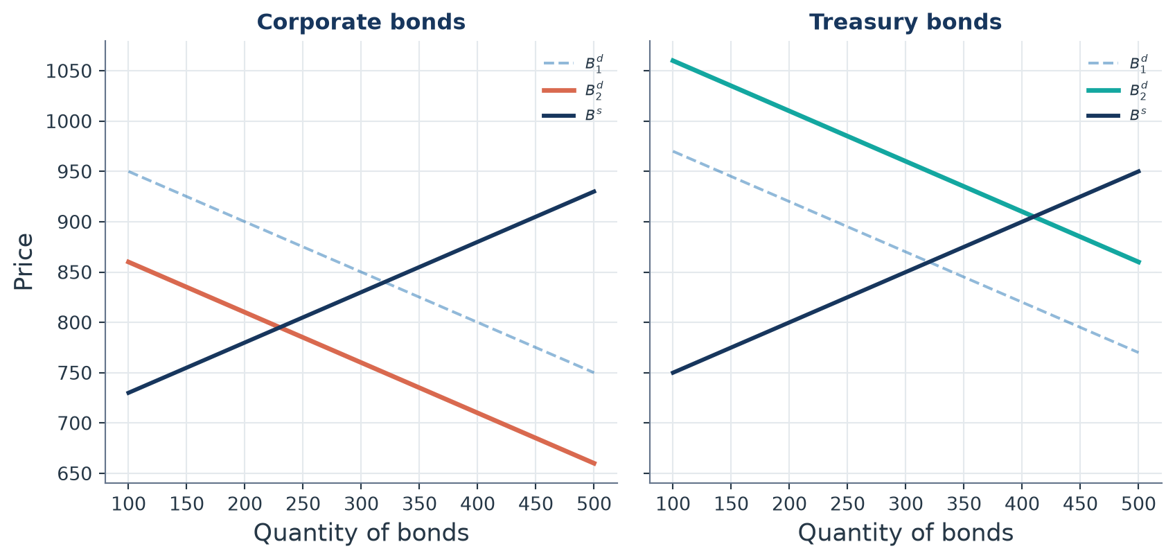
When corporate risk rises

Figure 6: A corporate-risk shock widens the spread against Treasury bonds

Corporate price ↓ (rate ↑) + Treasury price ↑ (rate ↓) = the spread (risk premium) widens.

Liquidity: the other component of the spread

A liquid asset can be converted to cash quickly and cheaply. Higher liquidity means higher demand — and a lower required rate.

That’s why the “risk premium” actually blends two things: default risk and liquidity. Textbooks call it the risk and liquidity premium.

The yield curve

A plot of the yield on bonds of equal risk and liquidity, across different maturities.

Any theory of the term structure must explain three facts:

1. Rates of different maturities move together over time.
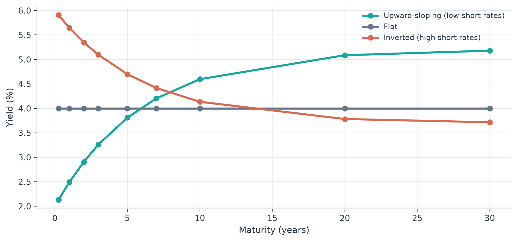
2. The curve is steeply upward-sloping when short rates are low, and inverted when they’re high.
3. The curve is, almost always, upward-sloping.

Shapes of the yield curve

Figure 7: Three typical shapes of the yield curve

An inverted curve has preceded almost every U.S. recession since 1960 — which is why markets watch it so closely.

Theory 1 · Pure expectations

The rate on a long-term bond = the average of the short-term rates expected over its life. \[ i_{nt}=\frac{i_t+i^e_{t+1}+i^e_{t+2}+\dots+i^e_{t+(n-1)}}{n} \] Key assumption: bonds of different maturities are perfect substitutes.

Example Expected 1-year rates over the next 5 years: 5%, 6%, 7%, 8%, 9%.

one_year_rates = [5, 6, 7, 8, 9]
expectations_curve = [np.mean(one_year_rates[:n]) for n in range(1,6)]
for n, r in zip(range(1,6), expectations_curve):
    print(f"{n}-year bond: {r:.2f}%")

1-year bond: 5.00%
2-year bond: 5.50%
3-year bond: 6.00%
4-year bond: 6.50%
5-year bond: 7.00%

Theory 2 · Market segmentation

Each maturity has its own market, unrelated to the others; the rate is set purely by the supply and demand for that maturity.

• ✅ Explains fact 3 (upward slope: more demand for short-term bonds → higher price → lower rate).

• ❌ Doesn’t explain facts 1 and 2 (rates moving together) because it assumes fully isolated markets.

Theory 3 · Liquidity premium

Combines the previous two: bonds are substitutes, but not perfect ones — investors demand a premium \(l_{nt}\) for holding long maturities. \[ i_{nt}=\underbrace{\frac{i_t+i^e_{t+1}+\dots+i^e_{t+(n-1)}}{n}}_{\text{expectations}}+\underbrace{l_{nt}}_{\text{increasing in }n} \]

It’s the dominant theory today because it’s the only one that explains all three facts simultaneously.

Comparing the theories with numbers

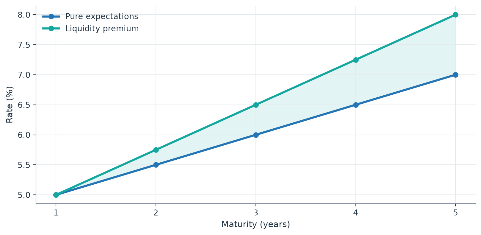
Same scenario Expected rates 5,6,7,8,9% + liquidity premiums of 0, .25, .5, .75, 1.0 pp

Figure 8: Pure expectations vs. liquidity premium: same expectations, different curve

The liquidity premium always tilts the curve upward — that’s why the “normal” curve slopes up even when no rate hikes are expected.

Synthesis: which theory explains what?

Fact to explain	Pure expectations	Segmentation	Liquidity premium
1. Rates move together	✅	❌	✅
2. Slope depends on the level of short rates	✅	❌	✅
3. Curve is usually upward-sloping	❌	✅	✅

Only the liquidity-premium theory passes all three tests — which is why it’s the standard framework in practice.

Wrap-up

Back to our opening question

Why does the U.S. government borrow almost for free, while Tesla doesn’t?

1. Default risk: the Treasury is (nearly) risk-free; Tesla isn’t.
2. Liquidity: Treasuries are the most liquid asset in the world.
3. Maturity: if Tesla issues at longer maturities, an additional liquidity premium stacks on top.

Quick retrieval check

Q1. If expected inflation rises, which way does bond supply shift? → Right (\(B^s\) rises, price falls, the rate rises).

Q2. A bond sells below its face value. Is its YTM higher or lower than the coupon? → Higher.

Q3. Which yield-curve theory explains all three empirical facts at once? → Liquidity premium.

Q4. Market interest rates rise. Which bond loses more value: a 2-year or a 20-year? → The 20-year (longer duration).

For next session

Case to prepare: Pick one Mexican corporate bond and one government bond (Cetes/Bonos M) of roughly the same maturity. Compare their rates and explain the spread using today’s material (risk + liquidity).

Suggested sources: Banxico (reference rates) and credit ratings from Trading Economics / the rating agencies.

References

Mishkin, F. S. & Eakins, S. G. Financial Markets and Institutions, chaps. 3–5.

Federal Reserve Bank of St. Louis (FRED) — series TB3MS, fetched live in this deck.